| Copyright July 1, 2000 | Vern Lindberg |
(a) Slopes and intercepts on log-log graph paper.8. Glossary
(b) Slope and intercept for semi-log graph.
Part I Uncertainties and Error Propagation |
Part III The Vernier Caliper |
The logarithmic scale has numbers (1,2,3 ... 9) printed on the axis. These numbers are spaced in proportion to the logarithms of the numbers. A cycle refers to one complete set of numbers from 1 to 10. We can have several cycles along one axis. It is important to purchase paper with the correct number of cycles for your application. Table 3 has a possible 2-cycle axis. (Some points are omitted for brevity.)
| Number | 1 | 2 | 3 | 4 | 6 | 8 | 10 | 20 | 30 | 40 | 60 | 80 | 100 |
| Log | 0.00 | 0.30 | 0.48 | 0.60 | 0.79 | 0.90 | 1.00 | 1.30 | 1.48 | 1.60 | 1.79 | 1.90 | 2.00 |
| Location of mark cm |
0.0 | 6.0 | 9.6 | 12.0 | 15.8 | 18.0 | 20.0 | 26.0 | 29.6 | 32.0 | 35.8 | 38.0 | 40.0 |
The numbers on the graph's log scale are marked 1, 2, 3 ... 9, 1, 2, 3, ... 1: you must use these numbers, but you can choose the decimal point. Thus a two cycle scale could start at 0.001 and go to 0.1 or it could start at 10 and go to 1000. Finding a slope on a semi-log or log-log plot takes some care. You must not compute rise/run as you did for linear paper.
Suppose we have data which could match a theoretical curve Y = A XM. For a log-log plot the slope is the value of the exponent M, and is computed as
 |
Eq. 3 |
On a log-log plot the slope, M, has no units. Either common (base 10) or natural logs can be used and give the same value of slope. The intercept, A, on a log-log plot is taken to be at the point where the horizontal variable has a value of 1. The value is read directly from the scale for the vertical axis. The units for the intercept are derived by looking at the form of the equation, Y = A XM, as is shown in the next example.
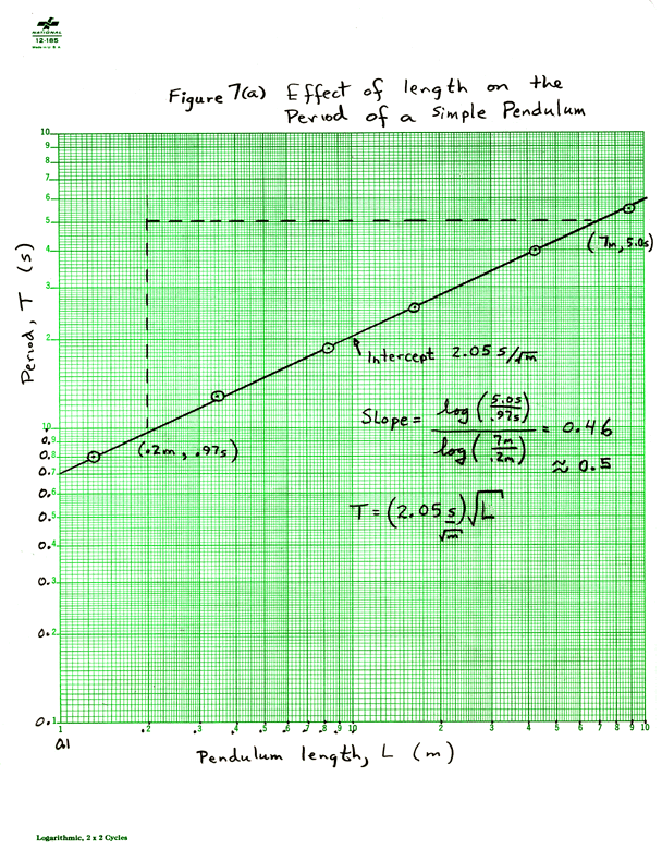
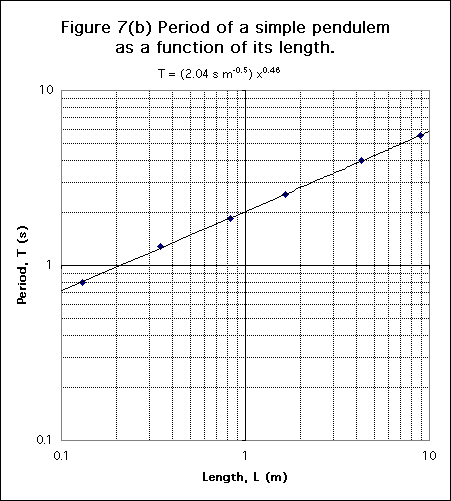
The data in Table 6 are plotted on Figure 7, with the slope calculation shown on the Figure 7(a). The slope here is 0.45 which is close to 1/2 meaning that the power may represent a square root.
| |
|
| |
|
|
|
|
|
|
|
|
|
|
|
|
|
|
|
|
The intercept in Figure 7 is 2.06. The units are derived by looking at the form of the equation, Y = A XM. Since Y (which really is T) has units of seconds and X (which really is L) has units of meters and the power M is a square root, the intercept is 2.06 s m-1/2. The equation is then
We check this by picking a length of L = 3.0 m and predict a period of T = 3.57 sec which agrees fairly closely with the value on the graph of 3.45 sec. The agreement would be closer if we used the exponent of 0.45 rather than the square root.
Figure 7(a) The hand drawn graph has been reduced to 90% of its original size.

Figure 7(b) This graph was done in Excel 98 on a Macintosh computer. Instructions on how to make this plot in Excel are included in the download. Download Excel 98 Source.

Suppose we expect our data to match a theoretical curve Y = A eM X. The slope, M, on a semi-log plot is computed by
 |
Eq. 4 |
The slope, M, on a semi-log plot has units which are the inverse of the units on the X-axis. Natural logs must be used here. The intercept, A, is the value where the line intersects the vertical axis at X = 0. It has the units of Y.
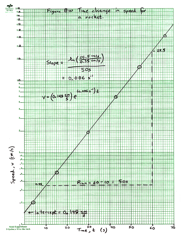
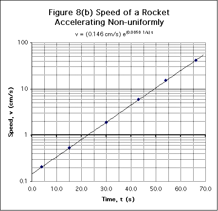
An example of a semi-log plot are the data in Table 5 which are plotted on Figure 8. The slope is found to be 0.0854 s-1and the intercept is found to be 0.150 cm/sec, as shown Figure 8(a). The equation for the rocket speed is then
![]()
We can check this equation by choosing a time, say 40.0 sec, and predicting the speed. The prediction is 4.57 cm/sec which agrees with the result on the graph of 4.60 cm/s.
| Time (sec) | Speed (cm/s) |
| 4.0 | 0.205 |
| 15.0 | 0.530 |
| 30.0 | 1.91 |
| 43.0 | 5.90 |
| 54.0 | 15.3 |
| 66.0 | 41.5 |
Figure 8(a) The hand drawn graph has been reduced from its original size.

Figure 8(b) This graph was done in Excel 98 on a Macintosh computer. Instructions on how to make this plot in Excel are included in the download.Download Excel 98 source.

| Abscissa | The horizontal axis. Usually the independent variable is plotted on the abscissa. See ordinate. |
| Axis Label | Each axis is labeled with the name of the variable, possibly the symbol of the variable, and the units. |
| Dependent Variable | The variable which we do not control, but only measure. Normally it is plotted on the vertical or ordinate. See independent variable. |
| Directly Proportional | A linear relationship with an intercept of zero. A graph of a linear relationship passes through the origin. |
| Error Bars | Vertical and/or horizontal marks indicating the possible range of values in a graph point. Usually one standard deviation long. |
| Graph Paper | Finely divided grid on which graphs can be drawn. Typically 10 squares to the inch, 20 squares to the inch, or 10 squares to the centimeter. Other types of graph paper exist. See quadrille paper. |
| Independent Variable | The variable over which we have control. Normally it is plotted on the horizontal or abscissa. |
| Intercept | For linear or semi-log graphs, the value of the ordinate (vertical) coordinate of a graph when the abscissa (horizontal) is zero. For log-log graphs, the value of the ordinate when the abscissa equals 1. It is also called the Y-intercept. It has the units of the ordinate. See slope, X-intercept, Y-intercept. |
| Log-Log Paper | Both axes are logarithmic scales. The divisions are marked on the paper and cannot be changed except to move the decimal point (tick mark 2 can be 0.02, 0.2, 2, 20, etc.) Special techniques are used to find slope and intercept. |
| Ordinate | The vertical axis. Usually the dependent variable is plotted on the ordinate. See abscissa. |
| Quadrille Paper | Usually a coarse grid (4 squares to the inch) useful for making engineering drawings, but not suitable for graphs. See graph paper. |
| Rise | The difference in the vertical coordinates of two points used to find the slope. The points should be far apart. See run. |
| Run | The difference in the horizontal coordinates of two points used to find the slope. The points should be far apart. See rise. |
| Scale | The choice of how many graph paper squares will represent 1 unit of the data. To allow easy reading of the graph choose 1 unit = 2, 5, or 10 squares. |
| Semi-Log Paper | Graph paper with one axis (usually the horizontal) that is linear and one (usually vertical) that is logarithmic. The divisions on the log scale are marked and cannot be changed except to move the decimal point. Special techniques are used to find slope and intercept. |
| Slope | The quantity M in the straight line equation Y = MX+B, it equals Rise/Run and usually has units. See intercept. Special techniques are used to find slope and intercept on graphs with log scales. |
| Tick Marks | Marks that extend into the margins of the graph paper to show exactly where the division label (number) is to be applied. See examples on graphs in this manual. |
| Title | The title of a graph should include a Figure number, and useful information about what is being plotted. It should not just repeat the axis labels. |
| X-Intercept | For linear or semi-log graphs, the value of the abscissa (horizontal) coordinate of a graph when the ordinate (vertical) is zero. For log-log graphs, the value of the abscissa when the ordinate equals 1. It has the units of the abscissa. See slope, Intercept, Y-intercept. |
| Y-Intercept | Another name for the intercept. See the definition there. See slope, Intercept, Y-intercept. |