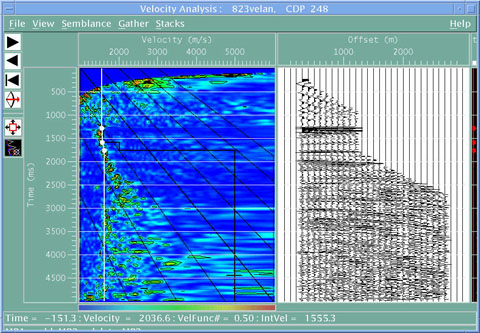
Velocity analysis showing picks with no moveout applied
ProMAX Lecture and Lab on Velocity Analysis
DEFINITIONS
RMS velocities and interval velocities Stacking(See Sheriff)
VRMS is the root mean square velocity. It is a type of weighted average
velocity. Weighted means that the thicker the layer in
which the ray travels, the greater the contribution to the final estimated VRMS
Interval Velocity: Velocity of a subsurface layer determined from travel
time through the layer of known thickness but in the
context of today's class it is derived using the Vrms and TWTT(s) to the top and
bottom of the layer using the Dix equation
Stacking Velocity: Velocity used for stacking data calculated from the
best-fit hyperbola to gather data through any of the
techniques that follow.
Background and Review to Velocity Analysis
Why do we use VRMS?
The equation for a hyperbola for the two layer case uses VRMS as a simplification for conditions of near vertical incidence.
If we know the VRMS down to the bottom of a layer and down to bottom of the previous
layer, we can estimate the individual
interval velocity of the last layer:
There are three velocities that we have seen in reflection seismology processing:
1. V true (simple for the first layer, but complex for more than one layer)
2. For real cases we tend to use a type of average velocity that fulfills the
equation for a hyperbola VRMS (another type of average
velocity),
3. Stacking Velocities In practice we use another velocity which is statistically
derived. It is the velocity that gives us the highest
amplitude signal in the data, and we can derive it in several ways:
1. Constant Velocity Analysis
Through trial and error we plot move out the traces at different times with a constant velocity (a Vrms)
|
Velocity analysis showing picks with no moveout applied |
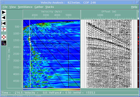
|
Velocity analysis showing picks with moveout applied |
2. Semblance Analysis
Measure the similarity of signals across a CDP gather and is expressed as:
the sum of energy across traces over an interval of time normalized
to the sum of energies in each trace
As the semblance increases across a gather, the stacking improves, and the output
signal preserves all the summed energy. Think that an
ideal signal will simply amplify the input:
This is done on a trial and error basis too.
Insert drawing: (handout)
Limitations
V stack is a cosmetic (looks good) best-fit velocity and it's derived assuming signals do not change shape with offset
V stack is distorted by processes that change the signal:
e.g. NMO stretch
e.g. near-critical phase changes
e.g. reflected signals can overlap
e.g. there's also random and coherent noise
e.g. we assume that the signal to noise ratio is the same in each trace and down
each trace although deep signals will have lower
frequencies and therefore lower resolution and greater error in estimating velocities.
Advantages
Multiples will stack at lower velocities than expected, and on average the signal/noise ration will improve.
ProMAX Lab
Aim: Interactively pick stacking velocities. Create interval velocity plot
1. Start ProMAX using Pro_all and go to Promax, then line 823
2. Copy the flow called velan to velan.yourname.
3. Make the following changes:
Disk Data Output ->
should become
Disk Data Output -> supergather.temp.yourname
Disk Data Input <- supergather
should become
Disk Data Input <- supergather.temp.yourname
Open Velocity Analysis and change
veloc.junk to:
veloc.junk.yourname
4. Execute this flow.
5.
(a) Under View select Tiles and then tick off CVS and Max. Semblance/IntervalVelocity
(b) Resize individual sub-windows
(c) Rescale traces in gather plot by adjusting the Trace Scale option to 5.0
Do this by going to View -> Trace Scaling -> gather scaling
1. Identify plots: Semblance plot, gather, CVS, Calculated interval velocity/Max Semblance
2. Interactively estimate the velocity of the first major reflection. As you move
your cursor the hyperbola is automatically calculated over
the gather plot.
3. Pick stacking velocities, using the semblance plot as your main reference.
Do you need to have a low velocity zone in your semblance
plot to produce a low velocity layer in the far right graph? How else
can you create a low velocity layer in the interval velocity plot?