|
PREAMBLE
Human beings are constantly involved with trying to classify
things into groups and then trying to understand the
similarities and differences between those groups. Often
the groups are already defined and we are interested in
discovering whether or not one group is really different from
another. In many cases this is import to us at the
personal level. For example, we have two groups one of
which takes drug A and the other which does not: are the results
similar or different. You measure a dozen different health
variables every day, such a temperature, blood pressure, pulse,
weight, calorie intake etc. You do this for a year and want to
know if there are any similarities or differences that are
related to changes during the week, month or whole year. The
answer to such questions are relatively easy to discover using
similarity indices.
A great deal of information is available to the general
public today in readily accessible form from digital
databases. Many of these are available at the local
library on CD or from the internet. Optical databases have
a potential shelf life much longer than the 150 years of acid
based printing paper and will become dominant in our libraries
in the next decade. However, the more useful aspects of
these data are not concerned so much with the ability to store
and access large general bodies of information, but with the
ease of access and ability to reduce the data, using available
statistical methods to answer questions pertinent to our lives.
Similarity indices are a group of statistical procedures that
are relatively easy to understand and present exciting
possibilities for real human-computer interaction. They
can provide a more objective experimental approach to
understanding data.
In order to analyze data quantitatively it is necessary to
understand the nature of data; how it should be collected; and,
how it can, and cannot, be used. One of the earliest
considerations for data analysis is designing a sampling plan to
ensure the information is reliable for the purpose for which it
is to be used. Different results may be obtained if different
sampling designs are employed; and, sometimes the question
answered by the results of a given sample study is not the same
as the question originally asked. A sampling plan is necessary
both for original studies or when the data is drawn from a large
database that already exists.
In designing a sampling plan to solve any specific problem
there are four procedural steps to be followed.
1. The problem must be clearly and reliably defined.
2. The sampling procedures must be specified prior to data
selection.
3. The measurement procedures must be stated and their limits
understood.
4. The technique for data analysis must be selected with due
regard to the first three procedural steps.
The purpose for undertaking any study must be clearly defined
at the very beginning. Defining the purpose implicitly defines
the problem and the population to be studied.
Problem definition also should examine the constraints within
which a solution must be found. Often a clear problem definition
shows it cannot be solved within its constraints. Scientific
constraints usually involve precision, accuracy, and
reliability; although, often the constraints of time, money and
personnel are more prominent in deciding whether, or not, to
attempt to solve a problem.
Precision is concerned
with dispersion, and accuracy is concerned with truth
(measured by a tendency to cluster around a central
point). However, the more general term reliability
pertains to the worth that an observer will place upon a result.
All of these concepts are related to an understanding of how a
sample relates to the target population that we are trying to
understand These concepts are pertinent to an understanding of
how s sample related to it's target population and how such
statistics as similarity indices are interpreted.
Similarity indices, as with statistical procedures in general,
often have been misused because of a lack of understanding of
basic statistical reasoning about population.
When sampling from a databank a
major assumption used is that the data is reliable. For
large data sets this assumption is often violated and error
checking must be performed. For example, in a test of reliability study of
the Oil and Gas Database from one of the US States Conservation
Department archives about six percent of the data records were
in error. This is consistent with an earlier study [1969]
when a test of reliability study was performed on
the accuracy of keypunched data [the old method of putting data
into the computer]. This study indicated that there was
almost a four percent error rate when data is put into a machine
by hand, and this four percent is repeated in both the first and
second set of corrections to the original data errors. Error
checking techniques, consistently applied, can remove most of
such errors.
TARGET POPULATION
The population under investigation must be clearly understood.
In all statistical investigations a sample is drawn from a
population of samples with the purpose of gathering information on
the Target population. My late friend John Griffiths noted
three types of target populations that we might be interested in
[Griffiths and Ondrick,1969].
The hypothetical population is the theoretical population that
should have been formed under the constraints of the model.
The existent population is the real population which now
exists and is the result of modification of the theoretical
population.
The available population is the readily available population
from which samples are drawn. Its relationship to the existent
population is generally a function of the cost (time, financial or
otherwise) required to collect random and representative samples
of the existent population.
A random sample is one in which each member of the sampled
population has the same chance of being selected as the sample, as
does any other member of the population. If the available
population is neither a random nor a representative sample of the
existent population it yields biased estimators which
cannot be adequately measured and gives conclusions that apply
solely to the samples taken and not to the population of
interest. It is therefore useless in answering questions
about the population.
To improve reliability and predictability in it is necessary to
ensure that the conclusions and interpretations actually apply to
the existent population. If the problem is to be solved
efficiently this must be accomplished during the designing of the
sampling plan. A failure to do this may result in conclusions
which do not apply to the target population.
SPATIAL VARIABILITY
Homogeneity in the
theoretical population is a crucial concept. If the
population to be sampled is homogenous we can draw our sample from
any part of it and be sure that we have a reasonable estimation of
the population. Unfortunately, most populations are not homogenous
but are structured.
When the population possesses structure one way to examine it
is to consider it a collection of homogenous
sub-populations. It then becomes necessary to randomly sample the
sub-populations, if such details are a necessary part of the
investigation. By necessity we have to assume homogeneity at our
lowest sampling level, but preferably should test for it.
In choosing the sampling design for a problem, one should
assume that the population is structured and sample accordingly at
the smallest affordable unit. If we adopt a sampling design that
assumes the population is not structured then our results may show
it is not structured: even if it is.
Because of inherent small scale variations in both space and
time one must consider that two kinds of samples exist. These are
spot samples and channel samples. In the earth for example, spot
samples are relatively small volumes of material derived from a
relatively small volume of the existent population. Channel
samples are linear strips of material which may extend centimeters
or meters. Channel samples are collected when one assumes
small scale structure in the existent population that are not of
interest to the problem. Channel samples cross the sub-populations
and give each its appropriate weight at the same time. A sample of
this type will contain no information on the structure within the
range of the sample. To obtain the latter it is necessary to
sample within the range of the sub-populations. Channel samples
will only be "best estimators" if they are appropriately
weighted to give the correct proportions of each sub-population in
the existent population. If this is done then a channel sample of
each unit will give a best estimator that is correctly
weighted for that unit. The same ideas apply for sampling
over time rather than space.
A special kind of sample is used in certain branches of earth
science. This is the ditch sample. This is a special kind of
channel sample used in subsurface geological studies. It is
derived from the cuttings produced from a rotary drilling rig. In
ditch samples the proportions of each sub-population cannot be
controlled. Various methods of "upgrading" the ditch
samples are used to improve the reliability of the cuttings.
Essentially, the aim is to permit the assumption that the cuttings
represent a reliable channel sample. Two common methods for
improving the reliability of the ditch cutting are back-picking
and front-picking of the sample prior to analysis. Back-picking
involves removing cuttings that are obvious contaminants whereas
front-picking involves selecting cuttings for analysis that are
believed to be representative of the interval being analyzed. We
are effectively biasing our sampling procedure by applying an
expert opinion to determining the composition of the sample.
Surprising the method usually works in that it gives testable
results. This type of sampling is rarely used outside earth
science but it has possibilities where samples are believed to
have been contaminated or distorted and they can be corrected by
recourse to expert opinion.
THE HARTAX PROGRAM
The various indices discussed in this manuscript were
implemented for single sample, linear and dual line analyses in
the HARTAX program written by
William B. Evans and myself in 1982, and previously unpublished.
The program is written in C and is both UNIX and MSDOS
based. A windows based module can be written if there is
sufficient interest.
THE MEASUREMENT OF DATA
Virginia Senders [1958], in her
delightfully common sense approach to Measurement and Statistics
notes that measurement is the process of assigning numerals to
objects [data] according to rules. Numerals, which are symbols and
not necessarily numbers, are assigned to objects using four
commonly used rules. The rule to use is implicit in the data
(objects). The most important point is that there is a direct
relationship between each rule and the degree to which the
properties of numbers (arithmetic) apply to the data. The rules
result in four different kinds of scales of measurement. These are
the nominal, ordinal, interval, or ratio scale of measurement. The
kind of scale upon which the data is measured is important because
it follows that the scale determines what kinds of
arithmetic manipulations can be performed on the data.
The term data types is used to imply the scale of
measurement that applies to the data. It must be emphasized that
the data type is important because it determines the kinds of
statistics that can be calculated from the sample. By setting
bounds on the appropriateness of statistical procedures it
determines the specific quantitative procedures that are
applicable to each problem.
NOMINAL DATA.
The nominal measurement scale is based on the idea of presence
and absence. It groups objects into classes because they have a
particular attribute, and makes no assumptions about any other
object in the classification. A modal class can be calculated. An
example is the naming of biological taxa or of colors.
ORDINAL
DATA.
The ordinal measurement scale groups objects into classes but
each class has a relative but none quantified relationship to each
other class. An example would be a relative scale of measurement
of the preservation of furniture into poorly preserved, moderately
preserved, well preserved and excellently preserved. A mode and a
median can be calculated.
INTERVAL DATA
The interval measurement scale groups objects into classes
which have an equal distance between each class but without any
regard to an absolute zero point. A mode, median, mean, standard
deviation and product-moment coefficients can be calculated.
Examples of interval data include calendar time and degrees
centigrade. In calendar time the time interval between 100 AD and
200 AD is the same as the time interval between 1700 AD and 1800
AD, but the year 200 AD is not twice as late in time as the year
100AD. The zero value was arbitrary and if we used a different
zero point then different relationships would hold amongst our
numerals. For degrees centigrade 20oC is not twice as
hot as 10oC. It should be noted that a similar argument
applies to the depth of a sample in the earth.
RATIO DATA
The ratio measurement scale is similar to the interval scale
but the true zero point is known. All available statistical
methods can be calculated for ratio scale data. Examples of ratio
data are the thickness of layer of rock in the earth,
degrees Kelvin, absolute time, and time intervals.
ATTRIBUTE TYPES
Attributes or variables are the fundamental objects measured on
a single sample, using one of the four scales of
measurement. Attributes are classified as continuous
or discrete according to the possible values they can
assume. If all definable values in an interval are possible then
the variable is continuous. If only a specific set of numbers may
be assumed within an interval then the variable is discrete.
The simplest way to visualize attribute measure is on a bar
chart [for discrete data categories] or a histogram / frequency
polygon [for continuous data]. Sometimes studies are undertaken
where a fixed number of attributes are used, and in such cases the
absence of an attribute is important and taken into account in
subsequent analysis. In other cases the absence of an
attribute is simply not recorded.
A further consideration is seen when we examine the attributes
in a data base. The variables may be primary, secondary,
redundant, or confounded.
Primary variables are measured attributes of an object that
represent fundamental information about that object i.e.
information that is not measured directly or indirectly by any
another variable in the data base.
Secondary variables are attributes of an object that are
derived from one or more primary variable(s). An example could be
higher taxonomic rank of organisms [e.g. Primates] derived from
the binomial [e.g. Homo sapiens]. In automated procedures
the secondary variables are derived from the primary variables by
passing the primary data through a filter. This filter is a
special computer program that must be written to perform the
specific procedure. Secondary variables always can be derived from
the primary variables within the database but may be kept within
the database as distinct attributes if their recalculation every
time they are needed would be inefficient.
Redundant variables are secondary attributes that do not
need to be kept in the database. The information contained in a
redundant variable already is present in one of the primary or
secondary variables.
Confounded variables are extremely common in studying the earth
sciences A confounded variable is a attribute which is known to be
a result of two or more primary attributes but the primary
attributes are not known e.g. the incidence of breast cancer in
different countries is influenced by numerous unknown variables.
Within the database the confounded variable must be handled as if
it were a primary variable. An important task of statistical
analysis of data is to partition a confounded variable into
its separate parts.
SPATIAL DIMENSION
The counting of attributes in a single sample is a multiple
attribute analysis. Such an analysis is merely an adjunct to
describing the sample. However, the interesting cases are
concerned with multiple sites. In many situations, such as
resource and environmental analysis as discussed in later
sections, spatial analysis is not concerned with the spatial
relationship of the attributes but with the spatial relationship
of the samples.
Procedures are the techniques that are applied to the
data during data analysis. Statistical procedures are a particular
set of techniques that are applied, and follow a general model:
Y = (something) + (error of measurement)
Where Y is said to be the dependent variable that is being
measured, and (something) is some relationship among the so-called
independent variables that control or predict Y.
An important aim of applying statistical procedures to a
database is data reduction. The aim of data reduction is to reduce
the amount of information to a size that can be interpreted by the
observer. There are numerous statistical procedures for analyzing
the data once it has been reduced. One way to understand how
to analyze a common set of problems is to group them into four
levels of complexity for quantitative data analysis. These
different levels of complexity will be illustrated by reference to
collections of biological and palaeontological data from surface
and subsurface samples. The respective databases are MDELTA
and KARROSS given in the Appendix
THE SINGLE SAMPLE PROBLEM
This is point analysis as might occur when examining a single
site or sampling station.
Within the KARROSS data base the single sample problem consists
of analyzing a record that in addition to its record number has
the variables Taxon (1) - Taxon (N). If one asks a group of good
taxonomists individually if they are good taxonomists the answers
will be yes. However, if you ask them if they will always agree,
with one another, on specific taxonomic identifications the answer
will be no. In fact there are various levels of taxonomic
stability depending upon the amount a work that has been
accomplished in the field, the diversity of training of the
taxonomist, the experience of the taxonomist and many other
factors. However, a basic assumption must be that the taxonomy is
stable. This often can be accomplished by a filter that
standardizes a taxonomic database (a synonymy filter). Hart and Fiehler [1971] and Hart [1972a] discussed
this problem.
Depending upon the data type the single sample problem simply
involves characterizing the sample by its statistics. The valid
interpretation is limited to diversity and relative abundance analysis. Minimally, a filter should be
available to determine the higher taxonomic grouping of the sample
data. Ideally, filter programs are available for determining the
age, the environment, and the similarity of the sample to other
samples in the database.
THE SINGLE LINE PROBLEM
This is linear analysis as
might occur when one takes samples along the course of a river or
from a borehole drilled into the subsurface. In biostratigraphic
terms this is the single well problem and involves multiple
samples, for which the depth is known, taken from a single
borehole. Depth may be measured on an ordinal, or interval scale.
An assumption is that the geological Law of Superposition holds
true, or that the database has been manipulated so that
superposition is true.
In such a study the most common problem to be solved is to
establish a single-well zonation within the constraints of the
International Code of Stratigraphic Nomenclature. In reality, the
problem is constrained by the resources that must be applied to
solve the problem (personnel, equipment, and time) and the
analytical capabilities of the system (of the observer and of the
hardware-software). This is because the results are
influenced by sample type [spot, channel, cutting], number of
individuals counted from the samples, etc.
The statistical problems associated with one well zonation are
concerned with sampling error. A one well zonation is precise but
of unknown accuracy or reliability. The sampling error in
biostratigraphic analysis is inherent in sample examination
(misidentifications, failure to observe a taxon that is present),
and sample spacing (failure to recognize confounding effects of
depth, lithology, environment; failure to apply the Rule of
Overlapping Ranges). These kinds of sampling error can be reduced
by the investment of more time in data gathering and/or the
application of error reduction techniques during the sampling
design and analysis phase of the data gathering.
Reliability is difficult to assess in the single line problem.
The confounding effects of lithology, depositional environment,
diagenesis. catagenesis, and climate have an influence on the
zonation but cannot be adequately assessed in the single well
problem. The Occurrence
Chart is the only real
biostratigraphic data to be analyzed. The conventional method of
analysis is to use the Range Chart.
This is an interpretation of the occurrence chart that visually
shows associations. Working with range charts the observer makes
decisions as to which associations are most important. Automated
techniques applicable to the single well problem use this
approach. The most reliable are the association techniques such as
cluster analysis, ordination analysis, unitary associations and
contour analysis. These are based on changes in an entire
assemblage as opposed to changes in a single taxon; and, their
function is to reduce the data to form where the zonation is less
biased.
Ranking and scaling algorithms are used to examine the
occurrence chart to extract preliminary zonation. Ranking is the process of placing a number of
individual samples in order according to some quality that they
all possess to a varying degree [Kendall, 1975]. Agterberg
and Nell [1982a] and Agterberg [1990] discuss some ranking
algorithms used in biostratigraphic analysis. In biostratigraphic
analysis the ranking of the 'tops' is an important process in
zonation. This is because most samples from boreholes are ditch
samples and the first occurrence of a taxon down a hole is its
most reliable occurrence [this is called it's top].
Because it is difficult to isolate the sources of variation
affecting the distribution of a taxon in time it is difficult to
know the true ranges of taxa. For this reason Agterberg [1983]
calls the results of applying a generalized ranking procedure the Optimal Sequence.
Scaling algorithms are
discussed by Agterberg and Nell [1982b] and Agterberg [1990].
These techniques calculate the distances between successive
stratigraphic events along a linear time scale. These distances
may be used in other procedures to seek assemblage zones [see
Hudson and Agterberg, 1982 using cluster analysis and dendrograms
for this purpose]
THE DUAL LINE PROBLEM
The dual line problem occurs when samples are taken along two
separate lines such as river channels. The use of similarity and
difference indices allows comparison of both samples within each
line and between each line. In
subsurface studies a special case of the dual line problem is
sectional analysis as might occur when two boreholes are sampled
and their samples compared. In geological terms this is the dual well
problem and is particularly important in providing a
biostratigraphic zonation that is generalized over both wells and
allows reliable biostratigraphic correlations. In sectional
analysis depth or time are the z - axis and a distance measure is
the x - axis. Compared with the single well problem the
zonation produced in a dual well problem should show decreased
precision but increased accuracy and reliability. It is important
to remember that the final decision concerning a zonation is made
by an individual observer.
The solution to the sectional problem should allow
partitioning of the confounded effects if replication of a
confounded variable occurs in wells. Sometimes the confounding can
be removed without further statistical analysis if ancillary
information is available. An additional difficulty in the two well
problem is the geographic variability that may be introduced, and
confounded with other effects. It may be possible to determine the
scale of geographic variability if all of the variation can be
correctly assessed. This is most likely if the correct sampling
design was used.
An important consideration in the sectional problem is the
difference between Matching and Correlation. Matching occurs when two wells exhibit
similar linear distribution of taxa and the distribution is not
controlled by time but is a result of other effects which are
confounded with depth e.g. lithofacies. Correlation occurs when
two wells exhibit similar vertical distribution of taxa that are
controlled by time. A knowledge of more general geological factors
may play a role in assessing the reliability of biostratigraphic
correlation. In general, a biostratigraphic (or
lithostratigraphic) correlation that is made along depositional
strike is more reliable than one made down depositional dip.
THE MULTIPLE LINE PROBLEM
This is a form of areal analysis when the samples can be
grouped on a single plane, and spatial analysis when they cut
different planes. When
the sets of samples are conceived as occurring within two
dimensional polygonal areas, and the analysis considers the
relationship of each polygon to it's surrounding polygons we are
dealing with classical areal analysis. Each polygonal area
is weighted according to it's nearness to all other polygonal
areas in the sampled universe. The comparison is a measure of both similarity
amongst attributes and distance apart of samples.
Samples or attributes should be
analyzed within the spatial framework of there existence when
location is important to the interpretation of their
relationships. In the geological subsurface the multiple line
problem is best seen as the multi-well problem and requires
spatial analysis of the data. The major difficulty that arises is
that the z - dimension is linear with depth but not with time but
it is time that controls the variations in most attributes. The x
- and y - axes are standard geographic coordinates. As the
number of wells increases in the problem-space the precision of
zonations is reduced and the accuracy increased. A general
consequence is that the number of biostratigraphic zones initially
decreases and then stabilizes. If the number of samples is large
enough the confounding effects may be isolated, in particular the
geographic effect may be partitioned so that the scale and
orientation of geographic variability is seen. An important
consideration in the multi-well study is that the amount of
confounding over a study of regional scale maybe so large that all
taxa may be shown to vary with regard to some effect other than
depth (or time). This was clearly seen in the 50 well study by
Hart [1972b] where the conclusion was:
there was no direct way to make detailed stratigraphic
correlations over regional distances using the percentage
abundance of miospore taxa. The reason for this may be due to any
one, or all of the sources of variation, acting upon miospores to
cause areal and temporal variation.
SAMPLING STATISTICS
In this section some of the simple statistical concepts
necessary to apply quantitative methods are introduced. The
approach is to consider the analysis of a single sample in which the measured variables are depth, and taxon[1] - taxon [N], in addition we include sample ID. From the early
discussion it is clearly important to determine the scale of
measurement of the data. This can generally be accomplished in a
simple way by asking the following questions about the data type.
1. Is one category simply different from
another category and that is all? If so the data is nominal.
2. Is one category bigger or better than another category? If
so the data is ordinal.
3. Is one category so-many units more than the next category?
If so the data is interval.
4. Is one category so-many times as big as the next category?
If so the data is ratio.
The statistical procedures that are appropriate for data
reduction under the different scales of measurement will be
discussed in terms of:
- distribution overview
,
- measures of central tendency,
- dispersion; and,
- position within the sample.
DENSITY
FUNCTIONS
The concept of a distribution is a central one in
statistical analysis of data. The PROBABILITY DENSITY FUNCTION
f(i) tells us for each value of i what the probability is of I
having that value. We can write the probability density function
for all possible values of i and if we draw a frequency graph of i
against f(i) we get a curve which defines the distribution of
the data. When a sample is compared with a population we are
comparing it to a specific distribution (either known or assumed).
The statistics calculated for a sample depends upon its
distribution.
The sampling distribution that should be used for
analyzing discrete data (whether nominal, ordinal or scalar), is
the multinomial distribution. If we have a population with
K categories: C1 C2 C3 C4.....Ck. Then for a sample size of
n (total count) with X (i) being the numbers in each
category by definition:
SUM (i=1,k) X (i) = n
eq1
In the case where k=2 the population has
only two categories. If p(i) is the proportion of X(i)
then:
X(2) = n - X(1)
eq2
and
p (i) = X(i)/n
eq3
Only one variable need be considered and this is called the
binomial variable. It is said to have a binomial distribution with
parameters n and p(i). The binomial distribution is
known for all values of p(i) and its characteristics
are well established. The expected value is:
E[X (i)] = np (i)
eq4
The dispersion is measured by the variance:
V[X (i)] = np (i)[1-p
(i)]
eq5
If n is large (>30) then a famous theorem
called the Central Limit Theorem says that the random
variable Z(i) defined as:
Z(I) = [X(i) - np(i)] /
SQRT[np(i){1-p(i)}]
eq6
will approximate a Normal or Gaussian
distribution. This is an important conclusion, for it means Normal
statistics can be used to analyze discrete data. It works very
well for n>30 and 0.2>p(i)<0.8. As p(i) moves away from
0.5 n must increase to remain a valid procedure. It should be
noted that Z(i) is in fact the observed value minus the expected
value then divided by the variance of the binomial distribution.
For the case where K>2 and p(i)>=0
then the sum of the proportions is 1 and the sum of x(i) is
n. With a large enough n and a random sampling each X(i)
has a binomial distribution and the population is said to have a multinomial
distribution. Under the appropriate conditions the variables
are approximately distributed as a Normal distribution.
Clearly, depending upon n and the values of
p(i) rests the method of analysis of nominal data. In one
case where the criteria for using a Normal distribution are met
then more powerful tests are available. In the other case direct
application of multinomial probability methods are used. Rigorous
application of this rule rejects the use of the more powerful
tests in many studies.
DECISION
RULE
If n>30 & 0.2>p(i)<0.8
then assume the Normal
Distribution. Otherwise directly apply Multinomial Probability
Methods.
NOMINAL DATA
|
|
APPROPRIATE STATISTICS FOR
NOMINAL DATA
[after Sander 1958, Stevens 1972] |
|
DISTRIBUTION OVERVIEW |
Bar Graph |
|
CENTRAL TENDENCY |
Mode |
|
DISPERSION |
Uncertainty |
|
POSITION |
Not appropriate |
|
In the simplest form
nominal data is binary, based on presence or absence of an
attribute ( using the base2 number system). The
analysis of ditch samples usually obtains data in a binary form.
Much more information can be derived from counts made on a higher
order number system e.g. base10. It should be noted
that the number system used is independent of the data type.
BINARY NOMINAL DATA
Table XX shows a flow chart for analyzing
nominal data. The basic information that can be obtained is a list
of the categories present (LIST), and the number of categories
present (CATS). Without the use of filter programs (AGE, ENVIR,
HITAX) to agglomerate or somehow tag the categories with another
characteristic nothing else can be done with the data.
MULTISTATE (DECIMAL) NOMINAL DATA
TABLE XX shows that additional data reduction procedures
are now available. Graphics in the form of a bar chart and a pie
chart are possible. Moreover, central tendency (mode) and
dispersion (uncertainty) can be estimated. Minimum, maximum
values and ratios, proportions and percentages of categories also
may be calculated. When data is measured on the nominal scale it
is not meaningful to describe the position of one observation
relative to other observations.
Dispersion
The measure of dispersion for nominal data is the uncertainty
statistic (H), measured in bits. This measures the average number
of binary decisions that must be made in order to determine the
category of an individual.
H = -SUM[p(i)LOG2p(i)] bits
eq7
where p is the proportion of cases in an
individual category. The higher H the greater the uncertainty. The
method is discussed in greater detail by Senders (1958).
Using the data A : .5 .5; B : .25 .5; C : .25
.5 the following is a worked example.
| CAT (i) |
p(i) |
-p(i)log2p(i) |
| A |
0.50 |
0.50 |
| B |
0.25 |
0.50 |
| C |
0.25 |
0.50 |
| |
|
SUM=1.5 |
An additional measurement is the relative
uncertainty H(rel). Whereas H describes the absolute uncertainty
or unpredictability of a distribution, the value H(rel) describes
the uncertainty as a comparison between the actual uncertainty and
the uncertainty that might exist if all counts were divided
equally amongst the various categories. The equation for relative
uncertainty is simple.
H(rel) = H / H(max)
eq8
If all counts are equally divided then:
H=H(max) and
H(rel)=1
eq9
but if only one category contains all counts then:
H(rel)=0.
eq10
For the case where all counts are equally divided:
H=log2(i).
eq11
Using the same example as above in which there are
three categories the expected values are 0.3 therefore:
H(max) = log2(3)
=1.5849 bits
eq12
H(rel) = 1.5000/1.5849
= .95 or 95% uncertainty
eq13
The measure of uncertainty (H) does not take into
account the ordering of the observation classes.
ORDINAL DATA
Distribution Overview
Multistate counts on
the ordinal data categories can be described by bar graphs when
discrete and by histograms when continuous. However, grouped
frequency, cumulative frequency, and percentage graphs also can be
used, because adjacent categories are related. It should be
remembered that the horizontal distances between points in such
graphs are arbitrary.
Central Tendency
Multistate counts on
discrete data can use the mode as a measure of central tendency,
however the median is generally a better predictor because it is
more stable than the mode, as more data is added. Moreover, the
mode is dependent upon the size of the class interval used and the
starting point of the individual classes.
Dispersion
Because measurements
on an ordinal scale take into account the order of the classes the
essential statistic for measuring dispersion is the Range.
This is measured as:
MAX-MIN or MAX-MIN+1
eq14
The variability can be
measured by Quartiles. The first quartile (Q1) contains 25%
of the observations, the second quartile (Q2) contains 50% of the
observations (the median), and the third quartile (Q3) contains
75% of the observations. The interquartile range (Q1-Q3) contains
50% of the measurements. An alternative is to give the Semi
interquartile range (Q3-Q1)/2=Q.
The units of measurement are those of the original observations.
Because of the problem associated with knowing the distance
between classes on the ordinal scale the calculated statistics of
quartile ranges are less preferable than an actual written
statement, such as "one fourth of the measurements had scores
below 15 microns and one fourth had scores above 125
microns)".
Position
When data is measured
on the nominal scale it is not possible to describe the position
of one observation relative to other observations. However, with
the ordinal scale measurement adjacent observations can be Ranked
from 1 to n simply by calling the lowest score 1, the second
lowest 2 and so on till n is reached. A more meaningful measure
actually takes into account the size of n and is the Percentage
rank measured by [RANK/n] * 100.
Computationally, this can be done more easily by:
{[OBS-MIN]/[MAX-MIN]}
* 100
eq15
If the data is
discrete the percentile rank can be found by the formula
%R=
{{[(OBS-L)*Fi]/I} + Fb}* {100/n}
eq16
L is lower class limit
of the interval within which the observation lies.
Fi is the number of
other observations in the class containing the observation to be
ranked.
Fb is the number of
observations below the class containing the observation to be
ranked.
n the number of
observations.
I is the width of the
class interval.
|
|
APPROPRIATE STATISTICS FOR
ORDINAL DATA
[after Sander 1958, Stevens 1972] |
|
DISTRIBUTION OVERVIEW |
Bar Graph [discrete]
Histograms (continuous)
Frequency Polygons
Cumulative Frequency
Cumulative Percentage |
|
CENTRAL TENDENCY |
Mode (discrete)
Median (more stable than mode) |
|
DISPERSION |
Inter-percentile Ranges |
|
POSITION |
Ranks
Percentile Ranks |
|
INTERVAL DATA
Distribution Overview
The general overview of multistate data can be
obtained using graphs in the same way as for nominal and ordinal
data. However, an important observation to be made is the amount
of Skewness and Kurtosis of the data. We can do this
because the horizontal distance between points on the graphs are
mathematically meaningful. Thus we can talk about the shape of the
distribution. Kurtosis measures the relative flatness or
peakedness of a distribution and skewness measures the tendency
for observations to clump at the lower (negatively skewed) or the
upper (positively skewed) end of the frequency distribution.
Skewness can be measured quantitatively but the value means very
little. Similarly, kurtosis can be precisely measured and related
to the normal curve, which has a value of 3. Curves are said to be
platykurtic, mesokurtic, or leptokurtic depending upon there
degree of flatness. It should be noted that superficially
mesokurtic curves with different standard deviations can simulate
both platy- and leptokurtic curves.
Central Tendency
The measure of central tendency for multistate
interval data is the ARITHMETIC MEAN.
Dispersion
The measure of dispersion for multistate data is
the standard deviation, and the average deviation
AD={[SUM:X-Xb:]/n}
eq17
For the average
deviation of the median substitute the median value for the mean.
Interestingly, this is a better estimate than the mean because it
leads to a smaller error in prediction. However, in general both
the average deviation of the mean and the average deviation of the
median are not rarely used because of the strength of the variance
as a measure of dispersion. Variance is the square of the
standard deviation (S), where:
S=SQRT{SUM[SQ(OBS-MEAN)]/(n-1)}
eq18
Position
The means of measuring relative position is the standard
score and normalized score. The fundamental standard
score is the z-score which relates the observation, the
mean and the standard deviation to one another by the equation
(OBS-MEAN)/S. In the normalized score each observation is assigned
its theoretical z-score according to its rank in the sample and
assuming a normal distribution. If the data is not normal then the
z-score and the percentile rank is given.
|
|
APPROPRIATE STATISTICS FOR
INTERVAL DATA
[after Sander 1958, Stevens 1972] |
|
DISTRIBUTION OVERVIEW |
Bar Graph [discrete]
Histograms (continuous)
Frequency Polygons
Cumulative Frequency
Cumulative Percentage
Skewness
Kurtosis |
|
CENTRAL TENDENCY |
Arithmetic Mean |
|
DISPERSION |
Average Deviation
Standard Deviation |
|
POSITION |
Standard Scores
Normalized Scores |
|
RATIO DATA
Distribution Overview
Ratio data uses the same techniques for
distribution overview as data measured on an interval scale. In
addition, transformations can be used to approximate the
theoretical distribution that the sampled date is assumed to
follow. By transforming the observations to a distribution that we
understand e.g. Normal, Poisson, we are able to correctly analyze
the data.
Central tendency
The measure of central tendency in ratio data is
estimated by the mode and mean but in addition the minor means
can be calculated. These are the Geometric mean, the Harmonic
mean and the Contra harmonic mean.
The geometric mean is the nth root of
the product of the observations.
G = n{SQRT[PROD(OBS)]}
eq19
The usual computational method is to calculate
LogG = {SUM[log(OBS)]}/n
eq20
and then get the anti-log to determine G. If a
transformation shows that the distribution is log-normally
distributed then the geometric mean is a better measurement of the
central tendency than is the arithmetic mean. The geometric mean
can never be used when at least one observation is
zero! It may be used to average ratios.
The harmonic mean is the reciprocal of the
mean of the reciprocals of the numbers. It should be used when the
reciprocals of the numbers are normally distributed.
HM=n[SUM(1/OBS)]
eq21
The contra harmonic mean is useful whenever a few
individual observations contribute a disproportionate amount to
the arithmetic mean; and, the relationship of these two means is a
measure of those contributions.
CHM={SUM[F*OB*OB]}/SUM[F*OB]}
eq22
An example follows. In this case there are 5
families of organisms and the number of species in each family is
given the table below.
|
# taxa/sample=T |
# of samples=OB |
T*OB |
| 4 |
10 |
40 |
| 3 |
10 |
30 |
| 2 |
10 |
20 |
| 1 |
10 |
10 |
| 0 |
10 |
0 |
| Totals |
50 |
100 |
Thus in 50 samples there are a total of 100 taxa!
The arithmetic mean is 2. However, we cannot conclude that the
average taxon comes from a two taxa sample. If we tabulate for
each taxon the number of taxa in the sample it came from we get
the following.
|
# taxa/sample=T |
# of samples |
T*OB |
| 4 |
40 |
160 |
| 3 |
30 |
90 |
| 2 |
20 |
40 |
| 1 |
10 |
10 |
| 0 |
0 |
0 |
| Totals |
100 |
300 |
Thus 100 taxa have 300 observations which is an
arithmetic mean of 3. This is the correct answer. The mean
calculated is actually the contraharmonic mean.
Dispersion
The dispersion is measured by the Variance
and by the Coefficient of variation. The CV is a pure
number measured in terms of the standard deviation and the mean.
CV=(100*S)/MEAN
eq23
Position
The position of one observation with respect to
the group is estimated using the same statistics as the interval
scaled data. In addition, an individual can be compared directly
as a ratio, often as an index number.
APPROPRIATE STATISTICS FOR
RATIO DATA
[after Sander 1958, Stevens 1972] |
| DISTRIBUTION
OVERVIEW |
Theoretical Distribution
Transformations to a distribution |
| CENTRAL
TENDENCY |
Geometric Mean
Harmonic Mean
Contra harmonic Mean
|
| DISPERSION |
Coefficient of Variation
Percent Variation
Decilog Dispersion
|
| POSITION |
Ratios
Index Numbers |
DATA
TRANSFORMATIONS
The ordinal
scale can be transformed by any increasingly monotonic function.
The interval scale allows multiplication by a constant. In general,
moving from an interval to a ratio scale of measurement does not add
much to the statistics that can be used. However, it does open up the
power of other mathematical techniques of analysis. Numerals from a
ratio scale have all the properties of real numbers and can be
raised to powers, have roots extracted, and reciprocal and logarithms
taken. Thus if a variable is not normally distributed then it can be
transformed to a form that is normally distributed and analyzed using
the powerful procedures of Normal statistics. The results can then be
transformed back into the real data set.
EQUITABILITY
In interpreting spatial data
it is often important to know how the specific abundance of attributes
and how they vary in a sample; and perhaps more importantly, how does
the abundance of attributes vary across sites. In many populations the
frequencies of occurrences of individuals having a particular attribute
in a sample are known to follow a specific statistical distribution. For
example, Gaussian, Lognormal, and Poisson distributions have all been
noted as being characteristic of certain populations. Functions are
readily available to test any sampled population to determine if it does
or does not fit a certain distribution, and standard univariate tests of
significance can be used to fail to reject the hypothesis that a
population fits a particular distribution. The types of equitability
measures considered herein are given in the following Table.
|
SINGLE
SITE EQUITABILITY INDICES
|
|
Index |
Applicability |
|
Grundy Exact Probability |
Ratio |
|
Relative Uncertainty |
Ratio |
|
Macintosh Ordination |
Ratio |
If the abundance of
attributes in a population is known, or assumed, to follow a specific
distribution then a measure of the abundance of a specific attribute is
fairly straightforward. For example, if it is assumed that the abundance
distribution of attributes is Lognormal then the frequency of occurrence
of the attributes from the sampled population can be assigned a location
under the Lognormal curve. Moreover, the shape of the sampled
distribution will allow the total number of attributes to be estimated.
Whether or not to include the unrepresented attributes [zero values]
depends on the analysis, and often a truncated distribution is used i.e.
the 0 abundance class is eliminated. One must decide whether or not zero
is a valid number in the dataset. Pielou [1969:203-220] has discussed
this for species relationships within a sample.
The ideas of evenness
and an even distribution provide a method for looking at how a sampled
population differs from a standard population. In this case the standard
assumes all categories are equally represented, and that an analysis
exists that can produce a statistic that estimates the difference
between the standard and the sampled population. Understanding such an
index may be difficult because sampling is from an available population
representing some theoretical population which has a real distribution
of categories. Almost certainly, this real distribution of categories
will not be the same as the standard population. What is needed,
therefore is a robust measure that is not influenced by the underlying
theoretical distribution.
GRUNDY
EXACT PROBABILITY INDEX
The exact probability method
of Grundy [1951], available for the discrete Lognormal distribution, is
the one we have implemented. This is the probability that an attribute
in a sample or collection of sites will be represented by r
individuals. The index is dependent upon the mode [m] and thus
influenced by sample size. The derived statistics of interest are the
estimates of the total number of attributes and the s2
[variance of the Lognormal curve].
 eq24 eq24 |
RELATIVE
UNCERTAINTY
Lloyd and Ghelandi [1964]
provided an early discussion of equitability. Relative uncertainty,
based upon the Shannon-Wiener function [Shannon & Wiener, 1949],
was used as a measure of sample equitability by Pielou[:233] who
gives the following formula for calculating Hmax.
 eq25 eq25 |
The index is influenced by
the evenness of the distribution and the number of attributes and as
such is slightly sample size dependent.
McINTOSH
EQUITABILITY INDEX
McIntosh [1967] provided an
ordination method for measuring equitability involving frequency and the
number of categories [K]. This is the McIntosh equitability index.
The evenness is a minimum when the attributes are evenly distributed.
|
 eq26 eq26
|
If the location of the
attribute or site categories are plotted in such a way that their
frequencies range from the high to the low values [or vice versa],
then the shape of the distribution is a visualization of the attribute
equitability [evenness] and site equitability. This is
shown in Figures x and x from which it is seen that diversity
and equitability can be illustrated together
.
|
ATTRIBUTE EVENNESS
|
SITE EVENNESS
|
 |
 |
DIVERSITY
Dispersion
observed in the categories of discrete
data sets for known
distributions is a measure of diversity. Robust measures of diversity are available. As Margalef [1958:50] pointed out a big drawback
when comparing samples that contain diverse types is that the process
of calculating the index is an attempt to
adjust a natural distribution to a simple mathematical expression of
more or less arbitrary form.
Pielou [1969, p.222] uses a definition of diversity that applies to
single samples and is concerned with variation in the number of
attributes and their abundances. This is
sample diversity and is related to the abundance [count] of
individuals [observations] in each attribute class, as was illustrated
in Figure x. It is the basis of the calculation of diversity indices
used by Pielou.
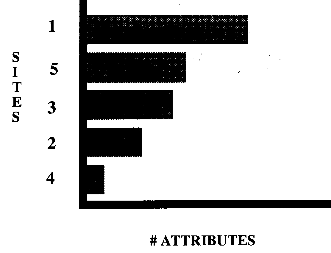
In addition, the term diversity is used to describe a characteristic of the
variation in either the number of sites or the number of attributes. Attribute diversity
is a count of how many sites are contained in each category of a set of
attributes; whereas, site diversity is a count of how many attributes occur in each
category of a set of sites. Figures 7 and 8 illustrate these concepts of diversity for a
site dataset using multistate counts. A major problem is that the
index generally depends upon sample size. The single site diversity
indices listed in the
Table below were implemented.
|
SINGLE SITE DIVERSITY
INDICES
|
| Shannon-Weiner |
Ratio |
|
McIntosh Ordination |
Ratio |
|
E. H. Simpson # 1 |
Ratio |
|
E. H. Simpson # 2 |
Ratio |
|
E. H. Simpson # 3 |
Ratio |
|
Margalet Diversity |
Ratio |
|
MacArthur Rarefaction |
Ratio |
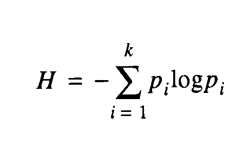
The basic diversity index is the uncertainty index [H] or the SHANNON-WIENER INDEX [Shannon & Wiener, 1949]. This index
relates the proportions [p] of cases in each category observed in the
available population.
eq27
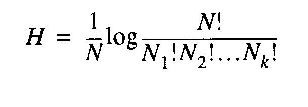
The units of H are those of the log such that log2 is in bits and log10 is in decits. The value is maximized when all categories are
represented in equal proportions and it can be used for all scales of
measurement.
eq28
In our analyses Stirling's Approximation is used to calculate the factorial.
eq29
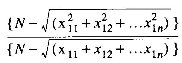
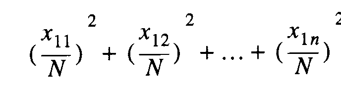
McIntosh [1967]
used an ordination method to estimate diversity for data measured on
interval or ratio scales. The McIntosh Ordination Index relates the number of categories and the frequency of
occurrence in each category using the following equation.
eq30
This provides a measure of diversity that is independent
of N
[Pielou, 1969:234]. The maximum value occurs when there is a single
category and the minimum when each category contains a single value.
This is an ordination technique because it's value is measured in K-category space with
coordinates x11...x1n.
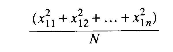
E. H. Simpson
[1949]
provided early examples of robust indices for measuring diversity based
on the probability that individuals sampled from a population will have
the same attribute e.g. will belong to the same species. He provided three formulae for calculating
diversity indices. SIMPSON INDEX # 1
measures single site diversity.
eq31
SIMPSON INDEX # 2 similarly measures single site diversity.
eq32
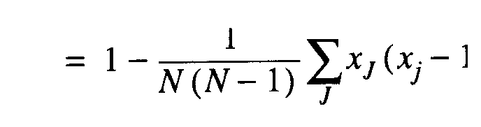
Pielou [1969:223]
discusses the basis of SIMPSON
INDEX # 3 and provides the
following formula.
eq33
Odum, Cantlar and Kornicker [1960] saw. in general, three approaches to diversity
indices. The first approach measures the rate of attribute
increase with additional sites i.e. the relationship of the cumulative
attributes against the log of their abundance. Margalef [1957] provides an example of this approach as the margalef diversity index. Margalef [1958] made on important contribution to diversity indices pointing out that information theory provides a diversity
index for a completely sampled population. Pielou
[1969:231-233] later gave an expanded discussion of this.
eq34
The second approach uses a Lognormal distribution and
was used by Preston [1948] using theoretical Lognormal frequencies and the
assumption that each category was represented by it's expected value. The Grundy
exact probability index discussed
earlier used this approach.
The third approach involves comparing the observed
abundances of categories with the log of
the rank. MacArthur [1957] used this method for calculating diversity in
non-overlapping ecological niches. The index relies on the number of
attributes and assumes a specific abundance for each category based on
the number of categories. Indeed, MacArthur
[1968] later rejected this index
after criticism by Pielou. Nevertheless, the index may have use for site
analysis. It is further discussed in Pielou
[1969:214-217].
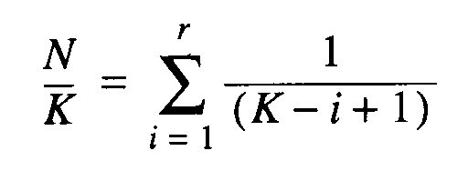
The MacArthur RAREFACTION INDEX is:
eq35
Where:
N = number of observations
K =number of attributes.
i =interval between
successively ranked attributes and the rarest attribute.
r =rank in the rarest attribute.
COMPARATIVE DIVERSITY INDICES
Comparative diversity indices
involve the calculation of a diversity index based on two samples. Those
indices implemented are listed in the Table below.
|
DUAL SITE DIVERSITY
INDICES
|
|
Austin & Orloci |
Ratio |
|
Bray & Curtis |
Ratio |
|
Canberra Metric |
Ratio |
|
G. G. Simpson # 1 |
Nominal |
|
G. G. Simpson # 2 |
Ratio |
|
G. G. Simpson # 3 |
Ordinal |
|
Crusafont & Santonja |
Ratio |
|
Kulczywski Community |
Ratio |
|
Whittaker |
Ratio |
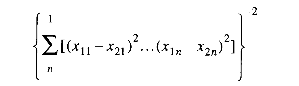
These dual site diversity indices when applied to multiple
samples produce a square matrix showing the index of all site pairs.
The basic calculation of such an index is indicated below using the AUSTIN & ORLOCI INDEX.
| |
Attribute 1 |
Attribute 2 |
Attribute 3 |
Attribute 4 |
|
Site 1 |
x11 |
x12 |
x13 |
x1n |
|
Site 2 |
x21 |
x22 |
x23 |
xx2n |
eq36
In this formulae:
(xp-xq)2 =1 if the
attribute is present at one of the sites;
(xp-xq)2 =0 if the
attribute is present or absent at both sites.
Here the Austin and Orloci index is the square root of a
simple count of the number of attributes present in one sample but
absent in another and as such is a difference measure.
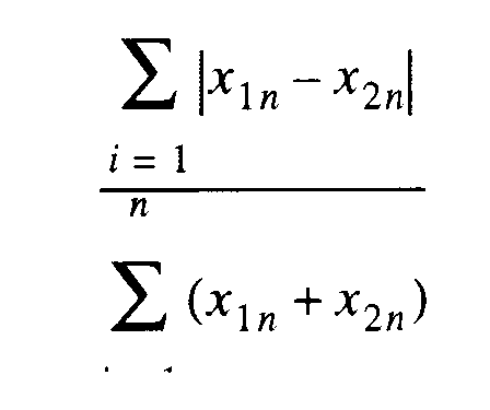
The Bray and
Curtis index is likewise a difference measure, ranging from 0
to +1 with +1 indicating the maximum difference.
eq37
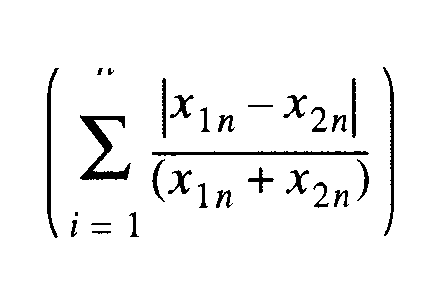
The Canberra
Metric likewise is a difference index. This
was used by Cook, Williams & Stephenson [1971] to analyze bottom communities.
eq38
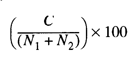
G. G. Simpson presented a series of dual sample
diversity indices for measuring site uniformity. The Simpson #1 index is a simple percentage index used for nominal
data.
eq39
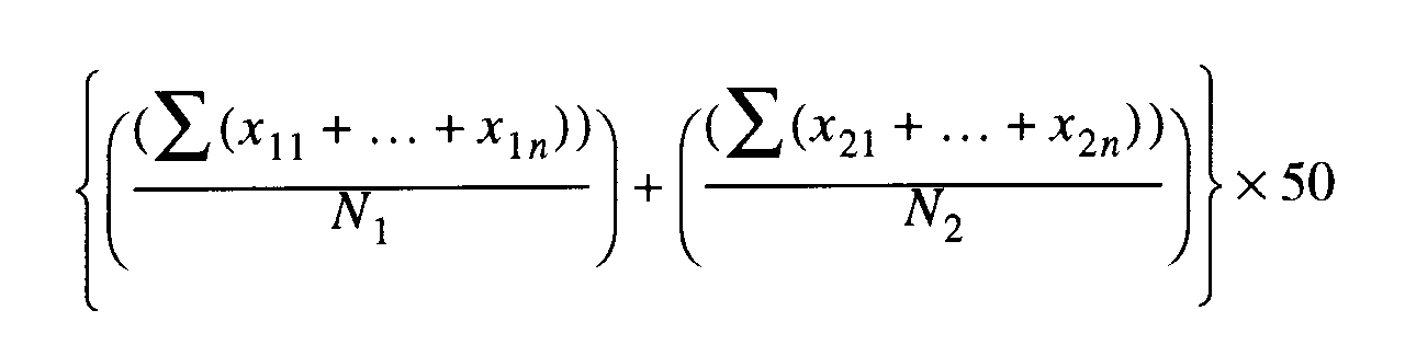
The Simpson #2 index can be used
for ratio data.
eq40
The Simpson
#3 index is used for ordinal data and uses the abundance rank of the attribute
at the site.
eq41
The CRUSAFONT
& SANTONJA INDEX is:
The KULCZYNSKI
COMMUNITY INDEX is:
The WHITTAKER
INDEX is:
SIMILARITY INDICES
Similarity is related to the variation between or
among objects. Variation is related to the
scale of measurement, and is the magnitude of the difference in
attribute [or sample] values, when two or more samples [or attributes]
are compared. There are a
variety of similarity indices that have been investigated and
published and these essentially can be classified according to the
scale of measurement of the data. In addition, specific kinds of
similarity indices have been developed for point, line, polygon, two
dimensional, and spatial datasets. Sokal & Sneath
[1963] provided a review of similarity indices and later Sneath &
Sokal [1973] reviewed the major classes of indices. The following Table list the similarity indices we have implemented. This figure indicates the highest scale of measurement of
the data to which each index can be applied.
|
Dice |
Nominal |
|
Fager |
Nominal |
|
Jacard |
Nominal |
|
Otsuka |
Nominal |
|
Simpson |
Nominal |
The indices for calculating attribute similarity over
sample space are based on the resemblance between two samples. Table 11
uses nominal data to illustrate a general similarity index. The sample
contingency table is generalized in Table 12 and from this
generalization a variety of similarity indices can be defined.
|
Table 11: FREQUENCY OF
ATTRIBUTES |
|
Attribute |
#1 |
#2 |
#3 |
#4 |
$5 |
|
Sample # 1 |
0 |
0 |
1 |
1 |
0 |
|
Sample # 2 |
1 |
0 |
1 |
1 |
0 |
|
Table 12: SIMILARITY TABLE |
|
Sample # 1 [Cij=0.4] |
| |
1 |
0 |
SUMS |
|
1 |
2 |
1 |
3 |
|
0 |
0 |
2 |
2 |
|
SUMS |
2 |
3 |
5 |
|
NOMINAL DATA TABLE |
|
Sample # 1 |
|
Sample # 2
|
|
1 |
0 |
|
|
1 |
a |
b |
a +
b |
|
0 |
c |
d |
c + d |
| |
a + c |
b + d |
p |
MATCHING INDICES
|
Roger & Tanimoto |
[N] |
|
Russel & Roe |
[N] |
|
Sokal & Michener |
[N] |
|
Hamman |
[N] |
|
Phi |
[N] |
|
Yule |
[N] |
ASSOCIATION INDICES
|
Braun-Blanquet |
[N] |
|
Kulczynski # 1 |
[N] |
DISTANCE INDICES
|
Minkowski metric |
[?] |
|
City Block metric |
[?] |
|
Euclidean metric [weighted] |
[?] |
|
Pearson's Chi-Sq |
[?] |
|
Mahalanobis |
[?] |
|
Calhoun non-metric |
[?] |
|
Lance & Williams non-metric |
[?] |
PROBABILISTIC
INDICES
SPATIAL PROXIMITY INDICES
|
Joint Count |
Ratio |
|
Geary |
Interval |
|
Moran |
Ratio |
|
Common Boundary |
[?] |
GENERAL INFORMATION INDICES
|
Shannon-Wiener |
|
|
Information #1 |
|
|
Information #4 |
|
|
Information #5 |
|
|
Information #6 |
|
|
Preston LogN |
|
|
Yule |
|
|
Resemblance |
|
|
Features of difference |
|
|
Squared distance |
|
APPLICATION OF THE INDICES
|
INDICES APPLIED TO RATIO DATA |
|
E. H. Simpson # 1 |
|
E. H. Simpson # 2 |
|
E. H. Simpson # 3 |
|
Fisher |
|
Brilliouin |
|
Sanders |
|
Margalet |
|
MacArthur # 1 |
|
MacArthur # 2 |
|
Measure of evenness |
|
Macintosh |
|
G. G. Simpson # 2 |
|
Austin & Orloci |
|
Bray & Curtis |
|
Crusafont & Santonja |
|
Kulczywski Community |
|
Cook |
|
Whittaker |
|
Moran |
|
Common boundary |
|
Shannon-Wiener |
|
Information # 1 |
|
Information # 4 |
|
Information # 5 |
|
Information # 6 |
|
Preston's LogN |
|
INDICES APPLIED TO INTERVAL DATA |
|
Geary |
|
INDICES APPLIED TO ORDINAL DATA |
|
G. G. Simpson # 3 |
|
INDICES APPLIED TO NOMINAL DATA |
|
Dice |
|
Otsuka |
|
Simpson |
|
Fager |
|
Jacard |
|
Simple |
|
Hamman |
|
Braun-Blanquet |
|
Kulczynski # 1 |
|
Yule Coefficient |
|
Coefficient of difference |
|
Sokal distance |
|
Rogers & Tanimoto |
|
Correlation ratio |
|
Phi |
|
Joint count statistics |
|
Yule |
|
Resemblance Equation |
|
Features of difference |
|
Squared Taxonomic distance |
|
G. G. Simpson # 1 |
VISUALIZATION METHODS
Essentially the method of
searching through pages of numbers derived from experimental results,
looking for anomalies that would support an hypothesis or present new
ideas is obsolete.Scientific visualization and especially three
dimensional visualization represents one of the most powerful
advancements in the application of computer technology to solving
scientific and real-life problems that has occurred in recent years.
Advances in printer and plotter technology has not only led to
camera-ready output allowing more rapid dissemination of results but
also has brought with it visualization tools that can be readily applied
during the phase of data analysis and at the computer screen. The
prospects and benefits of fast visualization technology means that it is
now possible to make computers present real world data in a graphical
format that is readily understandable and accessible by human operators.
Analytical software that allows concentration on the scientific
analysis enlarges our potential for discovering new
relationships. Defanti & Brown [1991] expressed this view as:
technical reality today and a
cognitive imperative tomorrow is the use of images. The ability of
scientists to visualize complex computations and simulations is
absolutely essential to ensure the integrity of analyses, to provoke
insights, and to communicate those insights with others.
VISUALIZATION
OF SITE DATA
The basic output from site
analysis is an unstructured table of similarity indices in which
each sample is compared with all others; and a bar chart showing the
abundance of each attribute in a sample. The results can be visualized
as an unstructured matrix of values but are better studied by further
statistical treatment such as the application of cluster, factor, or
discriminant function procedures.
VISUALIZATION
OF LINEAR DATA
The visualization of
similarities derived from linear analysis uses simple frequency
polygons, and pixel plots of the square matrix of
similarities. These matrices can be contoured as isoline maps.
Sectional data is readily visualized using isoline mapping procedures,
contoured block diagrams, and pixplots.
VISUALIZATION
OF AREAL DATA
Areal data can be best
visualized by choropleth maps and block diagrams.
VISUALIZATION
OF SPATIAL DATA
Three dimensional
visualization and voxel rendering are the appropriate ways to
examine the results of the analysis of spatial data. The natural
extension of the simple scientific visualization techniques is the use
of virtual reality to enhance the experience of the graphically defined
environment: the assumption being that virtual reality techniques can
improve the interpretative ability of the observer.
THE
PIXPLOT PROGRAM
REFERENCES
Austin
M. P. & Orloci L. 1966.
An evaluation of some ordination techniques. J. Ecology 54:217-227.
Bray
J. R. & Curtis J. T. 1957. An
ordination of the upland forest
communities of southern Wisconsin.
Ecol. Monograph.
Boots B.
N., & Getis A., 1988, Point
Pattern Analysis, Sage
Publications, London, 93 p.
Brillouin
L. 1962. Science and Information Theory. Academic Press New York 351 p.
Braun-Blanquet
1932. Plant Sociology:
the study of plant communities.
Translated by Fuller G. D. and Conrad H. S. McGraw-Hill
New York xvii+439
Cheetham
A. H. & Hazel J. E. 1969. Binary
[presence - absence] similarity coefficients. Journal of Paleontology 43[1130-1136].
Coleman
J. M., Hart G. F., Roberts H. H., Sen Gupta B. K., & Manning E.,1989. Gulf of Mexico Core
Study. School of Geoscience, Louisiana State University. Volumes 1 -
6.
Cook S.D., Williams W. T. & Stephenson W. 1971.
Computer analysis of Peterson's original data on bottom
communities. Ecol. Monograph.
42(4):387-415.
Crusafont Pairo M. & Truyols
Santonja J. 1958. Ensayo sobre el extablecimiento de una nueva
formula de semejanza fuanistica. Barcelona Inst. Biologia Aplicada
Publ. 28:87-94.
Defanti & Brown 1991.
Fager E.W. & McGowan J. A. 1963. Zooplankton attributes groups in the
North Pacific. Science 140:453-460
Fisher R. A. Corbet A. S.
& Williams C. B. 1943,
The relation between the number of attributes and the number of
individuals in a random sample of an animal population. Journ. Anim.
Ecol. 12:42-58.
Gordon A. D. Classification, Chapman & Hall, London,193 p.
Gleason H. A., 1922.
On the relation between species and
area. Ecology 3:158-162.
Griffiths and Ondrick, 1968
Griffiths and Ondrick, 1969
Hart G. F., 1965. The systematics and distribution of Permian miospores. University
of Witwatersrand Press, Johannesburg. 252 pages.
Hart G. F., 1972a.
Computerized
stratigraphic and taxonomic palynology for the lower Karroo miospores: a
summary. Second symposium on Gondwana Strat. e Paleont, Proceedings
and Papers: 541-542.
Hart G. F., 1972b. The Gondwana Permian
palynofloras. First symposium on Brazilian Paleontology. Rio de
Janeiro. An. Acad. Ciene., (1971), 43(Sup):145-185.
Hart G. F. & Fiehler J.,
1971. Kaross: a computer-based information
bank with retrieval programs for lower Karroo Stratigraphic Palynology. Geoscience
and Man, 3:57-64.
Imbrie
J.
and Purdy E. G. 1962. Classification
of modern Bahamian carbonate sediments. American Association of Petroleum
Geologists. Memoir 1:253-272
Jaccard P. 1908. Nouvelles
recherches sur la distribution florale. Bull. Soc. Vaud. Sci. Nat
44:223-270.
Kulczynski S. 1937. Zespoly
rosliln w pienincah - die pflanzen-assoziationen der pieninen.
Polon. Acad. des Sci. & Letters Cl. des Sci. Math. & Nat. Bull. Internatl. Ser. B
(suppl. II):57-203.
Lloyd H. A. and Ghelardi R.
J., 1964. A table for calculating the equitability component
of species diversity.
Journal of Animal Ecology 33:217-225.
MacArthur R. P., 1957.
On the relative abundance of bird
species.
Proceedings of the National Academy of Sciences of
Washington 43:293-295.
MacArthur R. P., 1965.
Note on Mrs.
Pielou's comments. Ecology
47:1074
MacArthur R. P., 1966.
Patterns of species diversity.
Biological Review 40:510-533
Margalef D. R., 1957.
Information theory in ecology.
General
Systems, 3:36-71
McIntosh R. P., 1967.
An index of
diversity and the relation of certain concepts to diversity.
Ecology
48:398-404.
Odum H. T.,
Cantlow J. E. and Kornicker L. S., 1960.
An organizational hierarchy
postulate for the interpretation of species individual distributions,
species entropy, ecosystem evolution and the meaning of a species
variety index.
Ecology
41:395-399.
Pielou C. 1966. The
measurement of diversity on different types of biological collections. Amer. Nat.
94:25-36.
Preston K. W., 1948.
The commonness and rarity of species.
Ecology 29:254-283
Ripley B. D., 1981.
Spatial Statistics. John Wiley & Sons, New York.252 p.
Ripley B. D., 1988.
Statistical Inference for Spatial
Processes. Cambridge
University Press, Cambridge, 148 p.
Sanders H. L. 1968. Marine benthic
diversity: a comparative study. Amer. Nat. 102:243-282.
Savage J. M. 1960. Evolution of
a peninsular herpetofauna Systematic.
Zoology 9:184-212
Senders V., 1958.
Measurement and Statistics,
Shannon C. E. & Weiner, 1963.
The Mathematical Theory of
Communication. University
of Illinois Press, Urbana, ILL.
Simpson E. H. 1949. Measurement of
diversity. Nature 163:688.
Simpson G. G. 1960. Notes on the
measurement of faunal resemblance. American J. Sci. 258-A:307-311.
Sneath P. H. A. & Sokal R. R.,
1973. Numerical Taxonomy. Freeman and Company, San Francisco. 573
p.
Sokal R. R. & Sneath P. H. A.
, 1963. Principals
of numerical taxonomy. Freeman
& Company, San Francisco. 359 p.
Sokal R. R. & Michener
C.D. 1958. A statistical method for evaluating systematic
relationships.
Univ. Kansas Sci. Bull. 38:1409-1438
Sorgenfrei T. 1959. Molluscan assemblages
from the marine middle Miocene of south Jutland and their environments. Denmark Geol. Unders. ser 2-79:2 vols. 503p.
Stephenson W., Williams W. T. & Lance G. N. 1968. Numerical
approaches to the relationships of certain. American swimming crabs
(Crustacea: Portunidea). Proc. U.S. Natl. Museum 124:1-25.
Whittaker R. H. 1952. A
study of summer foliage insect communities in the Great Smokey
Mountains. Ecol. Monogr.
22:1-44.
Whittaker R. H., 1965.
Dominance and diversity in
land plant communities. Science 147:250-260.
Williams
C. B.
1964. Patterns in the Balance of Nature. Academic
Press London. 324 p.
CATALOG OF INDICES
AUSTIN & ORLOCI INDEX
It is used for INTERVAL and RATIO data analysis
The formulae used is:
SQRT [ sum ( ( DNEG ) * ( DNEG ) )
]
REF:
AUSTIN M. P. & ORLOCI L. 1966 An evaluation of
some ordination techniques. J. Ecology 54:217-227.
BRAY & CURTIS INDEX
It is used for INTERVAL and RATIO data analysis
The formulae used is:
[ SUM |DNEG| ] / [ SUM ( DPOS ) ]
REF: BRAY J. R.
& CURTIS J. T. 1957 An ordination of the upland forest communities of southern Wisconsin.
Ecol. Monograph.
BRILLOUIN INDEX
It is used for INTERVAL and RATIO data analysis
The formulae used is:
[ LOG2 (N!) ] - [ SUM ( LOG2 (NI!)
) ]
REF: BRILLOUIN L. 1962 Science and Information
Theory. Academic Press
New York 351 p.
BRAUN-BLANQUET COEFFICIENT
Used for Q-mode analysis
It is used for NOMINAL data analysis
The formulae used is:
C / N2
where N1 < = N2
REF: BRAUN-BLANQUET 1932 Plant Sociology: the study of plant
communities. Translated by FULLER G. D. and CONRAD H. S.
McGraw-Hill New York xvii+439
COEFFICIENT OF DIFFERENCE
N.B. = (1-Braun-Blanquet Coefficient).
Used for R-mode analysis
It is used for NOMINAL data analysis
The formulae used is:
1 - ( C / N2 )
REF: SAVAGE J. M.
1960 Evolution of a peninsular herpetofauna Systematic. Zoology 9:184-212
COOK INDEX
syn: CANBERRA METRIC MEASURE.
It is used for INTERVAL and RATIO data analysis
The formulae used is:
SUM [ |DNEG| / ( CPOS ) ]
REF: COOK S.D., WILLIAMS W. T.
& STEPHENSON W. 1971 Computer analysis of Peterson's original data
on bottom communities. Ecol. Monograph. 42(4):387-415.
CORRELATION RATIO
Used for Q-mode analysis
It is used for NOMINAL data analysis
The formulae used is:
( C * C ) / ( N1 * N2 )
REF: SORGENFREI T. 1959 Molluscan assemblages from
the marine middle Miocene of south Jutland and their environments:
Denmark Geol. Unders. ser 2-79:2 vols. 503p.
CRUSAFONT & SANTONJA INDEX
It is used for INTERVAL and RATIO data analysis
The formulae used is:
[ 100 * IC * N1 * N2 ] / [ 2C ( I1
* N2 + I2 * N1 ) ]
REF: CRUSAFONT PAIRO M. & TRUYOLS SANTONJA J.
1958 Ensayo sobre el extablecimiento de una nueva formula de semejanza
fuanistica. Barcelona Inst. Biologia Aplicada Publ. 28:87-94.
REF: SIMPSON G. G. 1960 Notes on the measurement of faunal resemblance.
American J. Sci. 258-A:307-311.
DICE COEFFICIENT
syn: THE BURT
COEFFICIENT
syn:
THE
PIRLOT INDEX
Widely used in both Q- and R-mode analysis.
It is used for NOMINAL data analysis
The formulae used is:
(2C) / (N1 + N2)
REF: SOKAL AND SNEATH 1963 Principles of Numerical
Taxonomy: Freeman San Francisco. 359p.
E. H. SIMPSON INDEX # 1
It is used for INTERVAL and RATIO data analysis
The formulae used is:
SUM [ (NI * NI)/N ]
REF: SIMPSON E. H. 1949 Measurement of diversity Nature 163:688.
E. H. SIMPSON INDEX # 2
It is used for INTERVAL and RATIO data analysis
The formulae used is:
SUM [ (NI/N) * (NI/N) ]]
REF: SIMPSON E. H. 1949 Measurement of diversity Nature 163:688.
E. H. SIMPSON INDEX # 3
It is used for INTERVAL and RATIO data analysis
The formulae used is:
1-SUM [ (NI/N) * (NI/N) ]
REF: SIMPSON E. H. 1949 Measurement of diversity Nature 163:688.
FAGER COEFFICIENT
Used for Q-mode analysis
It is used for NOMINAL data analysis
The formulae used is:
[ C / SQRT ( N1 * N2 ) ] / 1 / 2 *
SQRT( N2 ) ]
where N1 < = N2
REF: FAGER E.W. & MCGOWAN J. A. 1963 Zooplankton attributes groups in the North
Pacific. Science 140:453-460
FISHER INDEX
It is used for INTERVAL and RATIO data analysis
The formulae used is:
{ N * [ 10 * EXP( (N1-N)/N1 ) ] }
/ { 1 - [ 10 * EXP( (N1-N)/N1 ) ] }
REF: FISHER R. A. CORBET A. S. & WILLIAMS C. B. 1943 The relation between the number of attributes and
the number of individuals in a random sample of an animal population.
Journ. Anim. Ecol. 12:42-58.
G. G. SIMPSON INDEX # 1
This is a percentage index.
It is used for NOMINAL data analysis
The formulae used is:
[ ( C ) / ( N1 + N2 ) ] * 100
REF: SIMPSON G. G. 1960 Notes on the measurement of faunal resemblance.
American J. Sci. 258-A:307-311.
G. G. SIMPSON
INDEX # 2
It is used for INTERVAL and RATIO data analysis
The formulae used is:
[ ( I1/ONEN ) + ( I2/TWON ) ] * 50
REF: SIMPSON G. G. 1960 Notes on the measurement of faunal
resemblance. American J. Sci. 258-A:307-311.
G. G. SIMPSON
INDEX # 3
It is used for NOMINAL and ORDINAL data analysis
The formulae used is:
[ 1 - SUM [ ( RANK1 - RANK2 ) * (
RANK1 -RANK2 ) ] ] / [ C [ ( C * C ) - 1 ] ]
REF: SIMPSON G. G. 1960 Notes on the measurement of faunal resemblance.
American J. Sci. 258-A:307-311.
HAMMAN COEFFICIENT
Used for R-mode analysis
It is used for NOMINAL data analysis
The formulae used is:
[ ( C + A ) - ( E1 + E2 ) ] / [ Nt
+ A ]
REF: SOKAL AND SNEATH 1963 Principles of Numerical
Taxonomy: Freeman San Francisco. 359p.
INFORMATION INDEX # 1
The formulae has not been implemented.
REF: PIELOU C. 1966 The measurement of diversity
on different types of biological collections. Amer. Nat.
94:25-36.
INFORMATION INDEX #4
The formulae has not been implemented.
REF: SANDERS H. L. 1968 Marine benthic diversity: a comparative study.
Amer. Nat. 102:243-282.
INFORMATION INDEX # 5
It is used for INTERVAL and RATIO data analysis
The formulae used is:
-SUM [ (NI/N) * LOGN (NI/N) ]
REF: MCARTHUR R. H. 1966 Patterns of attributes
diversity Biol. Rev. 40:510-533
INFORMATION INDEX # 6
It is used for INTERVAL and RATIO data analysis
The formulae used is:
-SUM [ (NI/N) * LOGE (NI/N) ]
REF: MCINTOSH R. P. 1967 An index of diversity and the relation of certain concepts to
diversity. Ecology
48:392-404.
JACCARD INDEX
Syn: COEFFICIENT OF COMMUNITY
Widely used in Q-mode analysis.
It is used for NOMINAL data analysis
The formulae used is:
C / (N1 + N2 - C)
REF: JACCARD P. 1908 Nouvelles recherches sur la
distribution florale. Bull.
Soc. Vaud. Sci. Nat 44:223-270.
KULCZYNSKI'S COMMUNITY INDEX
It is used for INTERVAL and RATIO data analysis
The formulae used is:
[ 2W ] / [ I1 + I2 ]
REF: KULCZYNSKI S. 1937 Zespoly rosliln w
pienincah - die pflanzen-assoziationen der pieninen. Polon. Acad. des
Sci. & Letters Cl. des Sci.
Math. & Nat. Bull. Internatl. Ser. B (suppl. II):57-203.
KULCZYNSKI'S FIRST COEFFICIENT
Used in both Q- and R-mode analysis.
It is used for NOMINAL data analysis
The formulae used is:
C / ( N1 + N2 - 2C )
REF: SOKAL AND SNEATH 1963 Principles of Numerical
Taxonomy: Freeman San Francisco. 359p.
KULCZYNSKI'S SECOND COEFFICIENT
Used in both Q- and R-mode analysis.
It is used for NOMINAL data analysis
The formulae used is:
[ C (N1 + N2) ] / [ 2 * N1 * N2 ]
REF: SOKAL AND SNEATH 1963 Principles of Numerical
Taxonomy: Freeman San Francisco. 359p.
MACARTHUR'S BROKEN STICK MODEL (FOR
NON-OVERLAPPING NICHES).
The formulae has not been implemented.
REF: MACARTHUR R. H. 1957 On the relative abundance of bird
attributes. Proc. Nat. Acad. Sci. 43:293-295.
MACARTHUR'S BROKEN STICK MODEL (FOR
OVERLAPPING NICHES).
The formulae has not been implemented.
REF: MACARTHUR R. H. 1957 On the relative abundance of bird attributes.
Proc. Nat. Acad. Sci. 43:293-295.
MARGALEF INDEX
It is used for INTERVAL and RATIO data analysis
The formulae used is:
[ N1-1 ] / [ LOGN (N) ]
REF: MARGALEF R. 1957 Information theory in
ecology. English Trans. Gen. System. 3:36-71
Macintosh INDEX
It is used for INTERVAL and RATIO data analysis
The formulae used is:
[ N1 - SQRT [ SUM (NI * NI) ] ] /
[ N - SQRT (N) ]]
REF: Macintosh R. P. 1967 An index of diversity and the
relation of certain concepts to diversity. Ecology 48: 398-404.
MEASURE OF EVENNESS
Used for Q-mode analysis
The formulae has not yet been implemented.
EQUITABILITY is a measure of the evenness of the
distribution of variables (taxa) in a sample
NUMBER OF FEATURES OF
DIFFERENCE
A special case of the Squared Taxonomic Distance of
Sokal.
It is used for NOMINAL data analysis
The formulae used is:
E1 + E2
REF: STEPHENSON W. WILLIAMS W. T.
& LANCE G. N. 1968. Numerical approaches to the relationships of certain. American swimming crabs (Crustacea: Portunidea). Proc. U.S. Natl. Museum 124:1-25.
OTSUKA COEFFICIENT
Use for BINARY DATA TYPES ONLY.
Used in both Q- and R-mode analysis.
This is a special case of the Coefficient of
Proportional Similarity (Imbrie and Purdy 1962).
SYN: THE OCHIAI COEFFICIENT
It is used for NOMINAL data analysis
The formulae used is:
C / SQRT ( N1 * N2 )
REF: SOKAL AND SNEATH 1963 Principles of Numerical
Taxonomy: Freeman San Francisco. 359p.
PHI COEFFICIENT
Used for Q- and R-mode analysis.
A special case of the Pearson Product-Moment
Coefficient.
An excellent statistic for Q-mode studies.
It is used for NOMINAL data analysis
The formulae used is:
[ ( C * A ) - ( E1 * E2 ) ] / SQRT[ N1 * N2 * ( E1 + A ) * ( E2 + A ) ]
REF: SOKAL AND SNEATH 1963 Principles of Numerical
Taxonomy: Freeman San Francisco. 359p.
PRESTON'S LOG NORMAL INDEX
The formulae has not been implemented.
REF: PRESTON F. W. 1948 The commonness and rarity of attributes. Ecol.
29:254-283
RESEMBLANCE EQUATION
Used for R-mode analysis
It is used for NOMINAL data analysis
The formulae used calculates 'Z' and is:
[ ( N1 / Nt ) ** (1 / Z) ] + [ (
N2 / Nt ) ** (1 / Z) ] = 1
REF: PRESTON F. W. 1962 The canonical distribution of commonness and
rarity:part II. Ecology 43:410-432
ROGERS AND TANIMOTO COEFFICIENT
Used for R-mode analysis
It is used for NOMINAL data analysis
The formulae used is:
[ C + A ] / [ Nt + A + E1 + E2 ]
REF: SOKAL AND SNEATH 1963 Principles of Numerical
Taxonomy: Freeman San Francisco. 359p.
SANDERS' INDEX
It is used for INTERVAL and RATIO data analysis
The formulae used is:
% of most abundant attributes.
REF: SANDERS H. L. 1968. Marine benthic diversity: a comparative study. Amer. Naturalist
102:243-282
SHANNON - WIENER INFORMATION
FUNCTION
SYN: INFORMATION INDEX # 3
It is used for INTERVAL and RATIO data analysis
The formulae used is:
-SUM [ (NI/N) * ( LOG2 (NI/N) ) ]
REF: SHANNON C. E.
& WEINER 1963 The Mathematical Theory of Communication. Univ. Ill. Press Urbana ILL.
SIMPLE MATCHING COEFFICIENT
Used in both Q- and R-mode analysis
Can be used only when there are 3 or more samples.
It is used for NOMINAL data analysis
The formulae used is:
(C + A) / (Nt + A)
REF: SOKAL R.R. AND MICHENER C.D. 1958 A
statistical method for evaluating systematic relationships:
Univ. Kansas Sci. Bull. 38:1409-1438
SIMPSON COEFFICIENT
Used for Q-mode analysis
It is used for NOMINAL data analysis
The formulae used is:
C / N1
where N1 < = N2
REF: SIMPSON G. G. 1943 Mammals and the nature of
continents. American J. Sci. 241:1-31
SOKAL DISTANCE
It is used for NOMINAL data analysis
The formulae used is:
SQRT[ ( E1 + E2 ) / ( Nt + A ) ]
REF: SOKAL AND SNEATH 1963 Principles of Numerical
Taxonomy: Freeman San Francisco. 359p.
SQUARED TAXONOMIC DISTANCE
The formulae is not implemented.
REF: SOKAL AND SNEATH 1963 Principles of Numerical
Taxonomy: Freeman San Francisco. 359p.
YULE COEFFICIENT
Used for R-mode analysis
It is used for NOMINAL data analysis
The formulae used is:
[ ( C * A ) - ( E1 * E2 ) ] / [ (
C * A ) + ( E1 * E2 ) ]
REF: SOKAL AND SNEATH 1963 Principles of Numerical
Taxonomy: Freeman San Francisco. 359p.
YULE INDEX
It is used for INTERVAL and RATIO data analysis
The formulae used is:
[N * N] / SUM [ NI (NI - 1) ]
REF: WILLIAMS C. B. 1964 Patterns in the Balance of Nature. Academic Press London.
324 p.
WHITTAKER'S INDEX
It is used for INTERVAL and RATIO data analysis
The formulae used is:
[ SUM |DNEG| ] / [ I1 + I2 ]
REF: WHITTAKER R. H. 1952. A study of summer foliage insect communities in
the Great Smokey Mountains. Ecol. Monogr. 22:1-44.